Pytorch 核心模块

• PyTorch 模块结构
• 核心数据结构——Tensor
• 张量的相关函数
• 自动求导核心——计算图
• Autograd——自动微分

1. Pytorch模块结构

所有虚拟环境中安装的库均在这个目录下\envs\库名\Lib\site-packages，并且虚拟环境是可以拷贝的，每个库文件夹下就是库中各个模块和一些通用的文件夹，下面会具体说明

pycache

该文件夹存放python解释器生成的字节码，后缀通常为pyc/pyo。其目的是通过牺牲一定的存储空间来提高加载速度，对应的模块直接读取pyc文件，而不需再次将.py语言转换为字节码的过程，从此节省了时间。

_C

它是辅助C语言代码调用的一个模块 PyTorch的底层计算代码采用的是C++语言编写，并封装成库，供pytorch的python语言进行调用。这一点非常重要，后续我们会发现一些pytorch函数无法跳转到具体实现，这是因为具体的实现通过C++语言，我们无法在Pycharm中跳转查看。

include

pytorch许多底层运算用的是C++代码，那么C++代码在哪里呢？ 在torch/csrc文件夹下可以看到各个.h/.hpp文件，而在python库中，只包含头文件，这些头文件就在include文件夹下。

lib

lib文件夹下包含大量的.lib .dll文件（分别是静态链接库和动态链接库），例如大名鼎鼎的cudnn647.dll（占435MB）， torchcuda.dll（940MB）。这些底层库都会被各类顶层python api调用。

autograd

该模块是pytorch的核心模块与概念，它实现了梯度的自动求导，极大地简化了深度学习研究者开发的工作量，开发人员只需编写前向传播代码，反向传播部分由autograd自动实现，再也不用手动去推导数学公式。

nn

pytorch开发者使用频率最高的模块，搭建网络的网络层就在nn.modules里边。

onnx

pytorch模型转换到onnx模型表示的核心模块。

optim

优化模块，深度学习的学习过程，就是不断的优化，而优化使用的方法函数，都暗藏在了optim文件夹中，进入该文件夹，可以看到熟悉的优化方法：“Adam”、“SGD”、“ASGD”等。以及非常重要的学习率调整模块，lr_scheduler.py。

utils

utils是各种软件工程中常见的文件夹，其中包含了各类常用工具，其中比较关键的是data文件夹，tensorboard文件夹，这些工具都将在后续章节详细展开。

torchvision库结构

安装Pytorch的时候也会装torchvision库，类似地，该库位于envs\pytorch1.10gpu\Lib\site-packages\torchvision，主要有以下模块。

datasets

这里是官方为常用的数据集写的数据读取函数，例如常见的cifar, coco, mnist,svhn,voc都是有对应的函数支持，可以方便地使用轮子，同时也可以学习大牛们是如何写dataset的。

models

这里是宝藏库，里边存放了经典的、可复现的、有训练权重参数可下载的视觉模型，例如分类的alexnet、densenet、efficientnet、mobilenet-v1/2/3、resnet等，分割模型、检测模型、视频任务模型、量化模型。

ops

视觉任务特殊的功能函数，例如检测中用到的 roialign, roipool，boxes的生成，以及focal_loss实现，都在这里边有实现。

transforms

数据增强库，transforms是pytorch自带的图像预处理、增强、转换工具，可以满足日常的需求。但无法满足各类复杂场景，因此后续会介绍更强大的、更通用的、使用人数更多的数据增强库——Albumentations。

2.核心数据结构——Tensor

在pytorch中，有两个张量的相关概念极其容易混淆，分别是torch.Tensor和torch.tensor。其实，通过命名规范，可知道torch.Tensor是Python的一个类, torch.tensor是Python的一个函数。通常我们调用torch.tensor进行创建张量，而不直接调用torch.Tensor类进行创建。 torch.tensor：pytorch的一个函数，用于将数据变为张量形式的数据，例如list, tuple, NumPy ndarray, scalar等。

张量的作用

tensor之于pytorch等同于ndarray之于numpy，它是pytorch中最核心的数据结构，用于表达各类数据，如输入数据、模型的参数、模型的特征图、模型的输出等。这里边有一个很重要的数据，就是模型的参数。对于模型的参数，我们需要更新它们，而更新操作需要记录梯度，梯度的记录功能正是被张量所实现的（求梯度是autograd实现的）。

Variable与Tensor

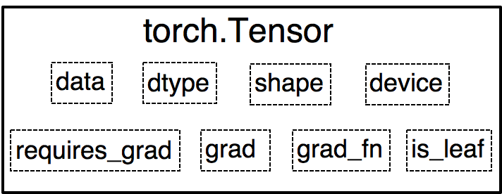
讲tensor结构之前，还需要介绍一小段历史，那就是Variable与Tensor。在0.4.0版本之前，Tensor需要经过Variable的包装才能实现自动求导。从0.4.0版本开始，torch.Tensor与torch.autograd.Variable合并，torch.Tensor拥有了跟踪历史操作的功能。虽然Variable仍可用，但Variable返回值已经是一个Tensor（原来返回值是Variable），所以今后无需再用Variable包装Tensor。 虽然Variable的概念已经被摒弃，但是了解其数据结构对理解Tensor还是有帮助的。Variable不仅能对Tensor包装，而且能记录生成Tensor的运算（这是自动求导的关键）。在Variable类中包含5个属性：data，grad，gradfn，isleaf，requires_grad

• data: 保存的是具体数据，即被包装的Tensor；
• grad: 对应于data的梯度，形状与data一致；
• grad_fn: 记录创建该Tensor时用到的Function，该Function在反向传播计算中使用，因此是自动求导的关键；
• requires_grad: 指示是否计算梯度；
• isleaf: 指示节点是否为叶子节点，为叶子结点时，反向传播结束，其梯度仍会保存，非叶子结点的梯度被释放，以节省内存。 从Variable的主要属性中可以发现，除了data外，grad，gradfn，isleaf和requiresgrad都是为计算梯度服务，所以Variable在torch.autogard包中自然不难理解。 但是我们的数据载体是tensor，每次需要自动求导，都要用Variable包装，这明显太过繁琐，于是PyTorch从0.4.0版将torch.Tensor与torch.autograd.Variable合并。

张量的结构

tensor是一个类，我们先来认识它有哪些属性，再去观察它有哪些方法函数可使用。 Tensor主要有以下八个主要属性，data，dtype，shape，device，grad，gradfn，isleaf，requires_grad。

• data：多维数组，最核心的属性，其他属性都是为其服务的;
• dtype：多维数组的数据类型；
• shape：多维数组的形状;
• device: tensor所在的设备，cpu或cuda;
• grad，gradfn，isleaf和requires_grad就与Variable一样，都是梯度计算中所用到的。 张量的属性还有很多，大家可以通过debug功能进行查看

3. 张量的相关函数

里面有上百个函数，这里只挑高频使用的进行记录，其他函数可参考Pytorch官方文档

直接创建

torch.tensor

torch.tensor(data, dtype=None, device=None, requiresgrad=False, pinmemory=False)

• data(array_like) - tensor的初始数据，可以是list, tuple, numpy array, scalar或其他类型。
• dtype(torch.dtype, optional) - tensor的数据类型，如torch.uint8, torch.float, torch.long等
• device (torch.device, optional) – 决定tensor位于cpu还是gpu。如果为None，将会采用默认值，默认值在torch.setdefaulttensor_type()中设置，默认为 cpu。
• requires_grad (bool, optional) – 决定是否需要计算梯度。
• pin_memory (bool, optional) – 是否将tensor存于锁页内存。这与内存的存储方式有关，通常为False。

import torch
import numpy as np
l = [[1., -1.], [1., -1.]]
t_from_list = torch.tensor(l)
arr = np.array([[1, 2, 3], [4, 5, 6]])
t_from_array = torch.tensor(arr)

torch.from_numpy

还有一种常用的通过numpy创建tensor方法是torch.from_numpy()。这里需要特别注意的是，创建的tensor和原array共享同一块内存（The returned tensor and ndarray share the same memory. ），即当改变array里的数值，tensor中的数值也会被改变。

torch.zeros

torch.zeros(*size, out=None, dtype=None, layout=torch.strided, device=None, requiresgrad=False) 功能：依给定的size创建一个全0的tensor，默认数据类型为torch.float32（也称为torch.float）。 主要参数： layout(torch.layout, optional) - 参数表明张量在内存中采用何种布局方式。常用的有torch.strided, torch.sparsecoo等。 out(tensor, optional) - 输出的tensor，即该函数返回的tensor可以通过out进行赋值，请看例子。 example:

import torch
o_t = torch.tensor([1])
t = torch.zeros((3, 3), out=o_t)
print(t, '\n', o_t)
print(id(t), id(o_t))

> >

tensor([[0, 0, 0],

[0, 0, 0],

[0, 0, 0]])

tensor([[0, 0, 0],

[0, 0, 0],

[0, 0, 0]])

4925603056 4925603056 可以看到，通过torch.zeros创建的张量不仅赋给了t，同时赋给了o_t，并且这两个张量是共享同一块内存，只是变量名不同。

torch.zeros_like

torch.zeroslike(input, dtype=None, layout=None, device=None, requiresgrad=False) 功能：依input的size创建全0的tensor。除了创建全0还有创建全1的tensor，使用方法是一样的

torch.full

torch.full(size, fillvalue, out=None, dtype=None, layout=torch.strided, device=None, requiresgrad=False) 功能：依给定的size创建一个值全为fill_value的tensor。

torch.full_like

torch.fulllike(input, fillvalue, out=None, dtype=None, layout=torch.strided, device=None, requiresgrad=False) torch.fulllike之于torch.full等同于torch.zeros_like之于torch.zeros，因此不再赘述。

torch.arange

torch.arange(start=0, end, step=1, out=None, dtype=None, layout=torch.strided, device=None, requires_grad=False) 功能：创建等差的1维张量，长度为 (end-start)/step，需要注意数值区间为[start, end)。 主要参数： start (Number) – 数列起始值，默认值为0。the starting value for the set of points. Default: 0. end (Number) – 数列的结束值。 step (Number) – 数列的等差值，默认值为1。 out (Tensor, optional) – 输出的tensor，即该函数返回的tensor可以通过out进行赋值。 example:

import torch
print(torch.arange(1, 2.51, 0.5))

torch.linspace

torch.linspace(start, end, steps=100, out=None, dtype=None, layout=torch.strided, device=None, requires_grad=False) 功能：创建均分的1维张量，长度为steps，区间为[start, end]。 主要参数： start (float) – 数列起始值。 end (float) – 数列结束值。 steps (int) – 数列长度(均分成几个)。 example:

print(torch.linspace(3, 10, steps=5))
print(torch.linspace(1, 5, steps=3))

torch.logspace

torch.logspace(start, end, steps=100, base=10.0, out=None, dtype=None, layout=torch.strided, device=None, requires_grad=False) 功能：创建对数均分的1维张量，长度为steps, 底为base。 主要参数： start (float) – 确定数列起始值为base^start end (float) – 确定数列结束值为base^end steps (int) – 数列长度。 base (float) - 对数函数的底，默认值为10，此参数是在pytorch 1.0.1版本之后加入的。 example:

torch.logspace(start=0.1, end=1.0, steps=5)
torch.logspace(start=2, end=2, steps=1, base=2)

torch.eye

torch.eye(n, m=None, out=None, dtype=None, layout=torch.strided, device=None, requires_grad=False)** 功能：创建单位对角矩阵。 主要参数： n (int) - 矩阵的行数 m (int, optional) - 矩阵的列数，默认值为n，即默认创建一个方阵 example:

import torch
print(torch.eye(3))
print(torch.eye(3, 4))

torch.empty

torch.empty(*size, out=None, dtype=None, layout=torch.strided, device=None, requiresgrad=False, pinmemory=False) 功能：依size创建“空”张量，这里的“空”指的是不会进行初始化赋值操作。 主要参数： size (int…) - 张量维度 pin_memory (bool, optional) - pinned memory 又称page locked memory，即锁页内存，该参数用来指示是否将tensor存于锁页内存，通常为False，若内存足够大，建议设置为True，这样在转到GPU时会快一些。

torch.empty_like

torch.emptylike(input, dtype=None, layout=None, device=None, requiresgrad=False) 功能：torch.emptylike之于torch.empty等同于torch.zeroslike之于torch.zeros，因此不再赘述。

torch.empty_strided

torch.emptystrided(size, stride, dtype=None, layout=None, device=None, requiresgrad=False, pinmemory=False) 功能：依size创建“空”张量，这里的“空”指的是不会进行初始化赋值操作。 主要参数： stride (tuple of python:ints) - 张量存储在内存中的步长，是设置在内存中的存储方式。 size (int…) - 张量维度 pinmemory (bool, optional) - 是否存于锁页内存。

依概率分布创建

torch.normal(mean, std, out=None)

功能：为每一个元素以给定的mean和std用高斯分布生成随机数 主要参数： mean (Tensor or Float) - 高斯分布的均值， std (Tensor or Float) - 高斯分布的标准差 特别注意事项： mean和std的取值分别有2种，共4种组合，不同组合产生的效果也不同，需要注意 mean为张量，std为张量，torch.normal(mean, std, out=None)，每个元素从不同的高斯分布采样，分布的均值和标准差由mean和std对应位置元素的值确定； mean为张量，std为标量，torch.normal(mean, std=1.0, out=None)，每个元素采用相同的标准差，不同的均值； mean为标量，std为张量，torch.normal(mean=0.0, std, out=None)， 每个元素采用相同均值，不同标准差； mean为标量，std为标量，torch.normal(mean, std, size, *, out=None) ，从一个高斯分布中生成大小为size的张量；

案例1

import 
mean = torch.arange(1, 11.)
std = torch.arange(1, 0, -0.1)
normal = torch.normal(mean=mean, std=std)
print("mean: {}, \nstd: {}, \nnormal: {}".format(mean, std, normal))

mean: tensor([ 1., 2., 3., 4., 5., 6., 7., 8., 9., 10.]),

std: tensor([1.0000, 0.9000, 0.8000, 0.7000, 0.6000, 0.5000, 0.4000, 0.3000, 0.2000,

0.1000]),

normal: tensor([ 1.3530, -1.3498, 3.0021, 5.1200, 3.9818, 5.0163, 6.9272, 8.1171,

9.0623, 10.0621]) 1.3530是通过均值为1，标准差为1的高斯分布采样得来， -1.3498是通过均值为2，标准差为0.9的高斯分布采样得来，以此类推

torch.rand

torch.rand(*size, out=None, dtype=None, layout=torch.strided, device=None, requires_grad=False) 功能：在区间[0, 1)上，生成均匀分布。 主要参数： size (int…) - 创建的张量的形状

torch.rand_like

torch.randlike(input, dtype=None, layout=None, device=None, requiresgrad=False) torch.randlike之于torch.rand等同于torch.zeroslike之于torch.zeros，因此不再赘述。

torch.randint

torch.randint(low=0, high, size, out=None, dtype=None, layout=torch.strided, device=None, requires_grad=False) 功能：在区间[low, high)上，生成整数的均匀分布。 主要参数： low (int, optional) - 下限。 high (int) – 上限，主要是开区间。 size (tuple) – 张量的形状。 example

print(torch.randint(3, 10, (2, 2)))

torch.randint_like

torch.randintlike(input, low=0, high, dtype=None, layout=torch.strided, device=None, requiresgrad=False) 功能：torch.randintlike之于torch.randint等同于torch.zeroslike之于torch.zeros，因此不再赘述。

torch.randn

torch.randn(*size, out=None, dtype=None, layout=torch.strided, device=None, requires_grad=False) 功能：生成形状为size的标准正态分布张量。 主要参数： size (int…) - 张量的形状

torch.randn_like

torch.randnlike(input, dtype=None, layout=None, device=None, requiresgrad=False) 功能：torch.rafndnlike之于torchrandn等同于torch.zeros_like之于torch.zeros

torch.randperm

torch.randperm(n, out=None, dtype=torch.int64, layout=torch.strided, device=None, requires_grad=False) 功能：生成从0到n-1的随机排列。perm == permutation

torch.bernoulli

torch.bernoulli(input, *, generator=None, out=None) 功能：以input的值为概率，生成伯努力分布（0-1分布，两点分布）。 主要参数： input (Tensor) - 分布的概率值，该张量中的每个值的值域为[0-1] example:

import torch
p = torch.empty(3, 3).uniform_(0, 1)
b = torch.bernoulli(p)
print("probability: \n{}, \nbernoulli_tensor:\n{}".format(p, b))
Copy

probability:

tensor([[0.7566, 0.2899, 0.4688],

[0.1662, 0.8341, 0.9572],

[0.6060, 0.4685, 0.6366]]),

bernoulli_tensor:

tensor([[0., 0., 1.],

[1., 1., 1.],

[1., 1., 1.]])

张量的操作

熟悉numpy的朋友应该知道，Tensor与numpy的数据结构很类似，不仅数据结构类似，操作也是类似的，接下来介绍Tensor的常用操作。由于操作函数很多，这里就不一一举例，仅通过表格说明各个函数作用，详细介绍可查看官方文档

scater_

scater是将input张量中的部分值进行替换。公式如下：

self[index[i][j][k]][j][k] = src[i][j][k]  # if dim == 0
self[i][index[i][j][k]][k] = src[i][j][k]  # if dim == 1
self[i][j][index[i][j][k]] = src[i][j][k]  # if dim == 2

设计两个核心问题：

1. input哪个位置需要替换？
2. 替换成什么？ 答：
3. 从公式可知道，依次从index中找到元素放到dim的位置，就是input需要变的地方。
4. 变成什么呢？ 从src中找，src中与index一样位置的那个元素值放到input中。

案例1：

>>> src = torch.arange(1, 11).reshape((2, 5))
>>> src
tensor([[ 1,  2,  3,  4,  5],
        [ 6,  7,  8,  9, 10]])
>>> index = torch.tensor([[0, 1, 2, 0]])
>>> torch.zeros(3, 5, dtype=src.dtype).scatter_(0, index, src)
tensor([[1, 0, 0, 4, 0],
        [0, 2, 0, 0, 0],
        [0, 0, 3, 0, 0]])

dim=0, 所以行号跟着index的元素走。其它跟index的索引走。 第一步：找到index的第一个元素index[0, 0]是0， 那么把src[0, 0]（是1）放到input[0, 0] 第二步：找到index的第二个元素index[0, 1]是1， 那么把src[0, 1]（是2）放到input[1, 1] 第三步：找到index的第三个元素index[0, 2]是2， 那么把src[0, 2]（是3）放到input[2, 2] 第四步：找到index的第四个元素index[0, 3]是0， 那么把src[0, 3]（是4）放到input[0, 3]

案例2：

>>> src = torch.arange(1, 11).reshape((2, 5))
>>> src
tensor([[ 1,  2,  3,  4,  5],
        [ 6,  7,  8,  9, 10]])
>>> index = torch.tensor([[0, 2, 4], [1, 2, 3]])
>>> index
tensor([[0, 2, 4],
        [1, 2, 3]])
>>> torch.zeros(3, 5, dtype=src.dtype).scatter_(1, index, src)
tensor([[1, 0, 2, 0, 3],
        [0, 6, 7, 8, 0],
        [0, 0, 0, 0, 0]])

dim=1：告诉input（零矩阵）的索引，沿着列进行索引，行根据index走。 index：2*3，告诉input（零矩阵），你的哪些行是要被替换的。 src：input要替换成什么呢？从src里找，怎么找？通过index的索引对应的找。 第一步：找到index的第一个元素index[0, 0]是0， 那么把src[0, 0]（是1）放到input[0, 0] 第二步：找到index的第二个元素index[0, 1]是2， 那么把src[0, 1]（是2）放到input[0, 2] 第三步：找到index的第三个元素index[0, 2]是4， 那么把src[0, 2]（是3）放到input[0, 4] 第四步：找到index的第四个元素index[1, 0]是1， 那么把src[1, 0]（是6）放到input[1, 1] 第五步：找到index的第五个元素index[1, 1]是2， 那么把src[1, 1]（是7）放到input[1, 2] 第六步：找到index的第六个元素index[1, 2]是3， 那么把src[1, 2]（是8）放到input[1, 3] 这里可以看到

• index的元素是决定input的哪个位置要变
• 变的值是从src上对应于index的索引上找。可以看到src的索引与index的索引保持一致的

案例3：one-hot的生成

>>> label = torch.arange(3).view(-1, 1)
>>> label
tensor([[0],
        [1],
        [2]])
>>> torch.zeros(3, 3).scatter_(1, label, 1)
tensor([[1., 0., 0.],
        [0., 1., 0.],
        [0., 0., 1.]])

第一步：找到index的第一个元素index[0, 0]是0， 那么把src[0, 0]（是1）放到input[0, 0] 第二步：找到index的第二个元素index[1, 0]是1， 那么把src[1, 0]（是1）放到input[1, 1] 第三步：找到index的第三个元素index[2, 0]是2， 那么把src[2, 0]（是1）放到input[2, 2] （one-hot的案例不利于理解scater函数，因为它的行和列是一样的。。。其实input[x, y] 中的x,y是有区别的，x是根据index走，y是根据index的元素值走的，而具体的值是根据src的值。）

张量的随机种子

随机种子（random seed）是编程语言中基础的概念，大多数编程语言都有随机种子的概念，它主要用于实验的复现。针对随机种子pytorch也有一些设置函数。

以上均是设置cpu上的张量随机种子，在cuda上是另外一套随机种子，如torch.cuda.manualseedall(seed)， 这些到cuda模块再进行介绍，这里只需要知道cpu和cuda上需要分别设置随机种子。

4.自动求导核心——计算图

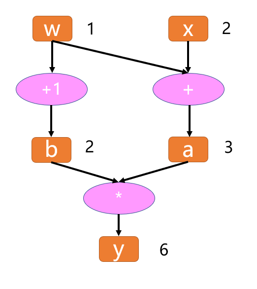
在学习自动求导系统之前，需要了解计算图的概念。计算图（Computational Graphs）是一种描述运算的“语言”，它由节点(Node)和边(Edge)构成。

计算图

根据官网介绍，节点表示数据和计算操作，边仅表示数据流向

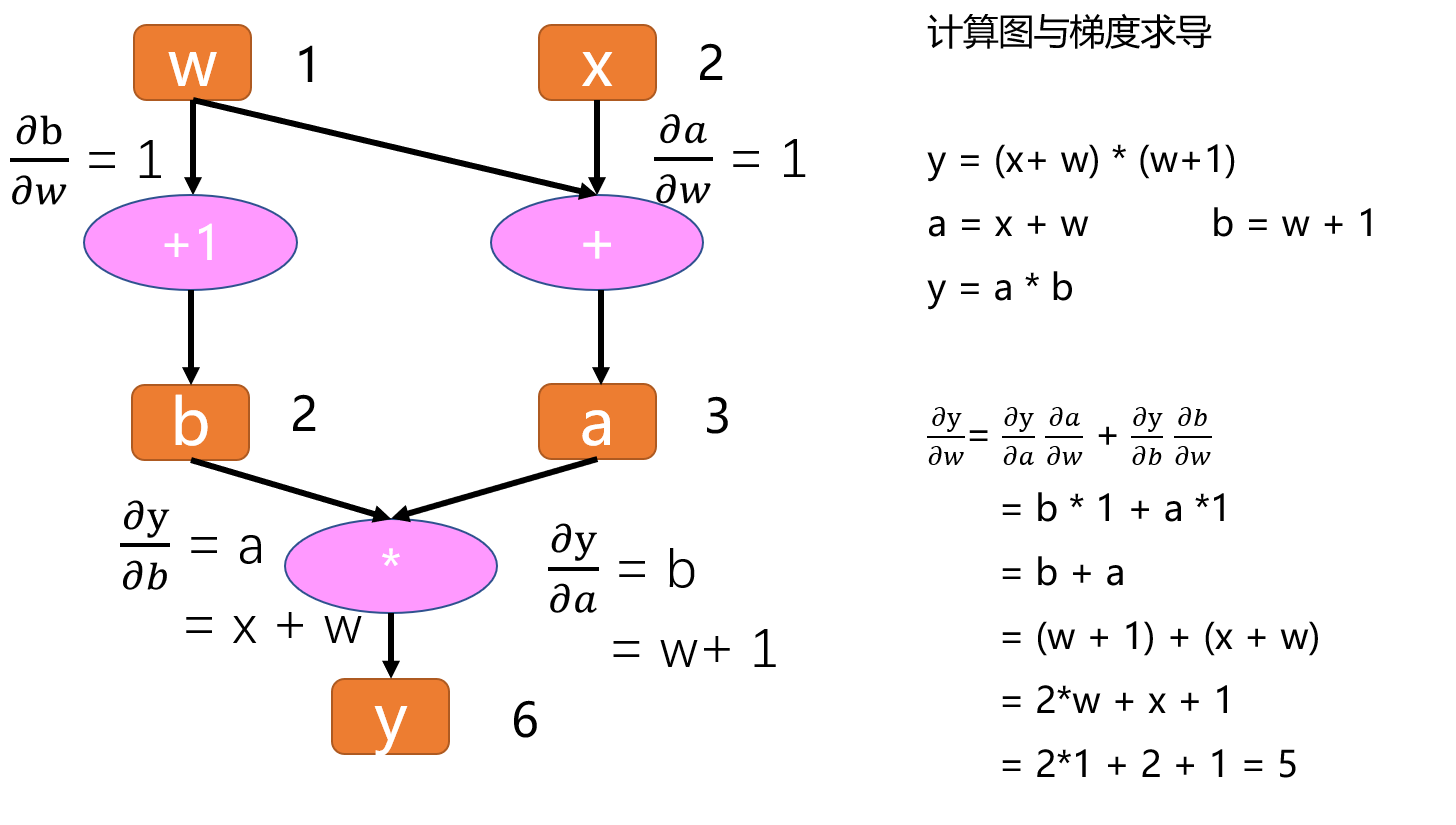
记录所有节点和边的信息，可以方便地完成自动求导，假设有这么一个计算：

y = (x+ w) * (w+1)

将每一步细化为：

a = x + w

b = w + 1

y = a * b

计算图求导

叶子节点

import torch

w = torch.tensor([1.], requires_grad=True)
x = torch.tensor([2.], requires_grad=True)

a = torch.add(w, x)
b = torch.add(w, 1)     # retain_grad()
y = torch.mul(a, b)

y.backward()
print(w.grad)
# 查看叶子结点
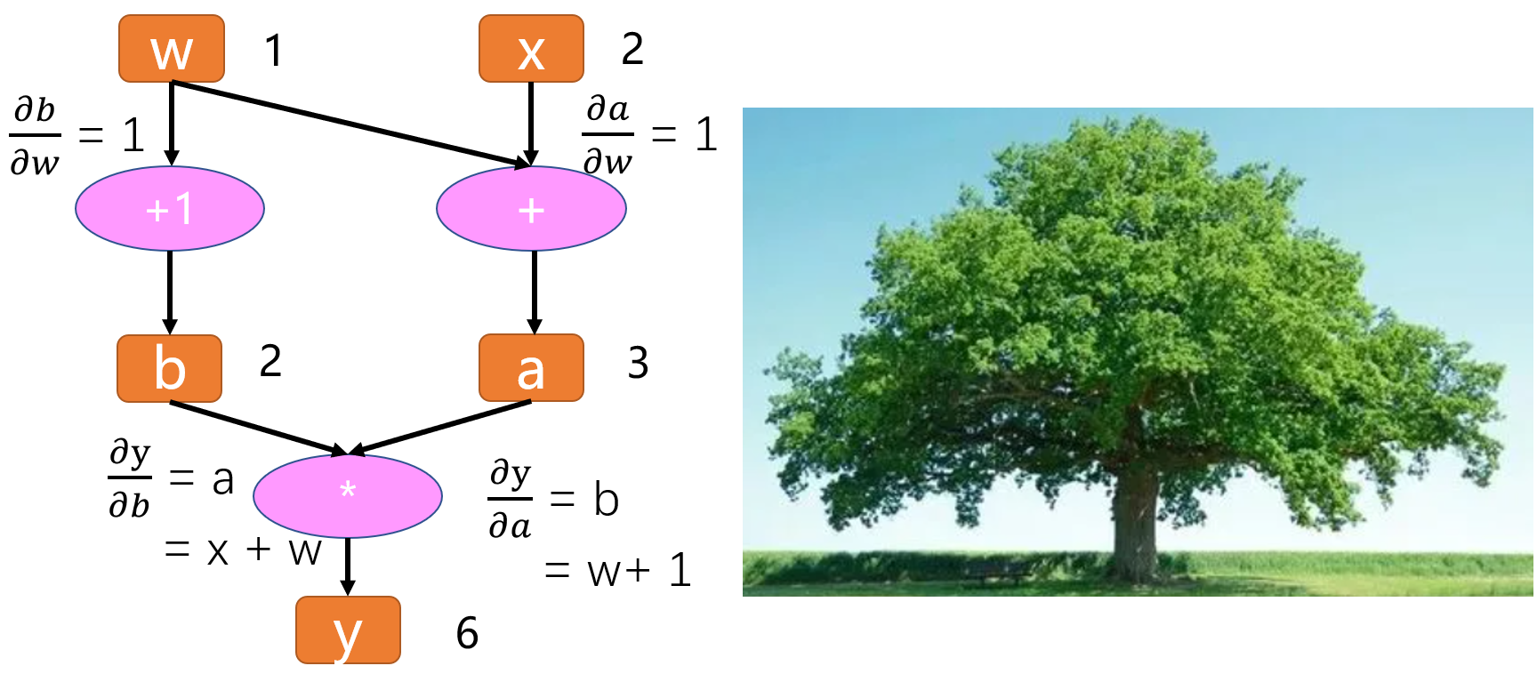
print("is_leaf:\n", w.is_leaf, x.is_leaf, a.is_leaf, b.is_leaf, y.is_leaf)
# 查看梯度
print("gradient:\n", w.grad, x.grad, a.grad, b.grad, y.grad)
# 查看 grad_fn
print("grad_fn:\n", w.grad_fn, x.grad_fn, a.grad_fn, b.grad_fn, y.grad_fn)

tensor([5.])

is_leaf: True True False False False

gradient: tensor([5.]) tensor([2.]) None None None

grad_fn: None None

静态图与动态图

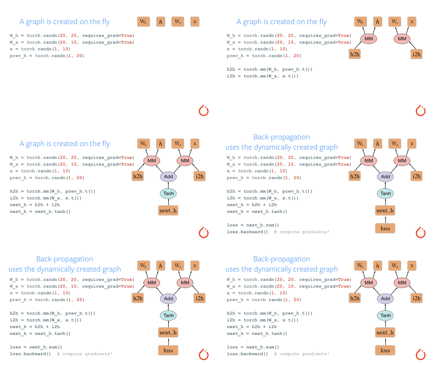
1. 易理解：程序按照编写命令的顺序进行执行
2. 灵活性：可依据模型运算结果来决定计算图 静态图优点：
3. 高效性：优化计算图，提高运算效率（但在gpu时代，这一点对于初学者而言可忽略不计） 缺点：
4. 晦涩性：需要学习 seesion, placeholder等概念，调试困难

5.自动微分

了解计算图后，我们可以开始学习autograd。 以上上图为例，在进行h2h、i2h、nexth、loss的计算过程中，逐步搭建计算图，同时针对每一个变量（tensor）都存储计算梯度所必备的gradfn，便于自动求导系统使用。当计算到根节点后，在根节点调用.backward()函数，即可自动反向传播计算计算图中所有节点的梯度。这就是pytorch自动求导机制，其中涉及张量类、计算图、grad_fn、链式求导法则等基础概念。

autograd 的使用

autograd的使用有很多方法，这里重点讲解一下三个，并在最后汇总一些知识点。更多API推荐阅读官方文档

• torch.autograd.backward
• torch.autograd.grad
• torch.autograd.Function

torch.autograd.backward

backward函数是使用频率最高的自动求导函数，没有之一。99%的训练代码中都会用它进行梯度求导，然后更新权重。 loss.backward()就可以完成计算图中所有张量的梯度求解。 虽然绝大多数都是直接使用，但是backward()里边还有一些高级参数，值得了解。 torch.autograd.backward(tensors, gradtensors=None, retaingraph=None, creategraph=False, gradvariables=None, inputs=None)

• tensors (Sequence[Tensor] or Tensor) – 用于求导的张量。如上例的loss。
• grad_tensors (Sequence[Tensor or None] or Tensor, optional) – 雅克比向量积中使用，详细作用请看代码演示。
• retaingraph (bool, optional) – 是否需要保留计算图。pytorch的机制是在方向传播结束时，计算图释放以节省内存。大家可以尝试连续使用loss.backward()，就会报错。如果需要多次求导，则在执行backward()时，retaingraph=True。
• create_graph (bool, optional) – 是否创建计算图，用于高阶求导。
• inputs (Sequence[Tensor] or Tensor, optional) – Inputs w.r.t. which the gradient be will accumulated into .grad. All other Tensors will be ignored. If not provided, the gradient is accumulated into all the leaf Tensors that were used to compute the attr::tensors. 补充说明：我们使用时候都是在张量上直接调用.backward()函数，但这里却是torch.autograd.backward，为什么不一样呢？ 其实Tensor.backward()接口内部调用了autograd.backward。 请看使用示例

retain_grad参数使用

对比两个代码段，仔细阅读pytorch报错信息。

####  retain_graph=True
import torch
w = torch.tensor([1.], requires_grad=True)
x = torch.tensor([2.], requires_grad=True)

a = torch.add(w, x)
b = torch.add(w, 1)
y = torch.mul(a, b)  

y.backward(retain_graph=True)
print(w.grad)
y.backward()
print(w.grad)
tensor([5.])
tensor([10.])

运行上面代码段可以看到是正常的，下面这个代码段就会报错，报错信息提示非常明确：Trying to backward through the graph a second time。并且还给出了解决方法： Specify retain_graph=True if you need to backward through the graph a second time 。 这也是pytorch代码写得好的地方，出现错误不要慌，仔细看看报错信息，里边可能会有解决问题的方法。

####  retain_graph=False
import torch
w = torch.tensor([1.], requires_grad=True)
x = torch.tensor([2.], requires_grad=True)

a = torch.add(w, x)
b = torch.add(w, 1)
y = torch.mul(a, b)

y.backward()
print(w.grad)
y.backward()
print(w.grad)
tensor([5.])

RuntimeError: Trying to backward through the graph a second time (or directly access saved tensors after they have already been freed). Saved intermediate values of the graph are freed when you call .backward() or autograd.grad(). Specify retain_graph=True if you need to backward through the graph a second time or if you need to access saved tensors after calling backward.
Copy

grad_tensors使用

w = torch.tensor([1.], requires_grad=True)
x = torch.tensor([2.], requires_grad=True)

a = torch.add(w, x)     
b = torch.add(w, 1)

y0 = torch.mul(a, b)    # y0 = (x+w) * (w+1)    dy0/dw = 2w + x + 1
y1 = torch.add(a, b)    # y1 = (x+w) + (w+1)    dy1/dw = 2

loss = torch.cat([y0, y1], dim=0)       # [y0, y1]

grad_tensors = torch.tensor([1., 2.])

loss.backward(gradient=grad_tensors)    # Tensor.backward中的 gradient 传入 torch.autograd.backward()中的grad_tensors

# w =  1* (dy0/dw)  +   2*(dy1/dw)
# w =  1* (2w + x + 1)  +   2*(w)
# w =  1* (5)  +   2*(2)
# w =  9

print(w.grad)
tensor([9.])

torch.autograd.grad

torch.autograd.grad(outputs, inputs, gradoutputs=None, retaingraph=None, creategraph=False, onlyinputs=True, allow_unused=False) 功能：计算outputs对inputs的导数 主要参数：

• outputs (sequence of Tensor) – 用于求导的张量，如loss
• inputs (sequence of Tensor) – 所要计算导数的张量
• grad_outputs (sequence of Tensor) – 雅克比向量积中使用。
• retaingraph (bool, optional) – 是否需要保留计算图。pytorch的机制是在方向传播结束时，计算图释放以节省内存。大家可以尝试连续使用loss.backward()，就会报错。如果需要多次求导，则在执行backward()时，retaingraph=True。
• create_graph (bool, optional) – 是否创建计算图，用于高阶求导。
• allow_unused (bool, optional) – 是否需要指示，计算梯度时未使用的张量是错误的。

此函数使用上比较简单，请看案例：

import torch
x = torch.tensor([3.], requires_grad=True)
y = torch.pow(x, 2)     # y = x**2

# 一阶导数
grad_1 = torch.autograd.grad(y, x, create_graph=True)   # grad_1 = dy/dx = 2x = 2 * 3 = 6
print(grad_1)

# 二阶导数
grad_2 = torch.autograd.grad(grad_1[0], x)              # grad_2 = d(dy/dx)/dx = d(2x)/dx = 2
print(grad_2)
(tensor([6.], grad_fn=<MulBackward0>),)
(tensor([2.]),)

torch.autograd.Function

有的时候，想要实现自己的一些操作（op），如特殊的数学函数、pytorch的module中没有的网络层，那就需要自己写一个Function，在Function中定义好forward的计算公式、backward的计算公式，然后将这些op组合到模型中，模型就可以用autograd完成梯度求取。

这个概念还是很抽象，平时用得不多，但是自己想要自定义网络时，常常需要自己写op，那么它就很好用了，为了让大家掌握自定义op——Function的写法，特地从多处收集了四个案例，大家多运行代码体会Function如何写。

案例1： exp

案例1：来自 https://pytorch.org/docs/stable/autograd.html#function 假设需要一个计算指数的功能，并且能组合到模型中，实现autograd，那么可以这样实现 第一步：继承Function 第二步：实现forward 第三步：实现backward

注意事项：

1. forward和backward函数第一个参数为ctx，它的作用类似于类函数的self一样，更详细解释可参考如下： In the forward pass we receive a Tensor containing the input and return a Tensor containing the output. ctx is a context object that can be used to stash information for backward computation. You can cache arbitrary objects for use in the backward pass using the ctx.saveforbackward method.
2. backward函数返回的参数个数与forward的输入参数个数相同, 即，传入该op的参数，都需要给它们计算对应的梯度。

import torch
from torch.autograd.function import Function

class Exp(Function):
    @staticmethod
    def forward(ctx, i):

        # ============== step1: 函数功能实现 ==============
        result = i.exp()
        # ============== step1: 函数功能实现 ==============

        # ============== step2: 结果保存，用于反向传播 ==============
        ctx.save_for_backward(result)
        # ============== step2: 结果保存，用于反向传播 ==============

        return result
    @staticmethod
    def backward(ctx, grad_output):

        # ============== step1: 取出结果，用于反向传播 ==============
        result, = ctx.saved_tensors
        # ============== step1: 取出结果，用于反向传播 ==============


        # ============== step2: 反向传播公式实现 ==============
        grad_results = grad_output * result
        # ============== step2: 反向传播公式实现 ==============


        return grad_results

x = torch.tensor([1.], requires_grad=True)  
y = Exp.apply(x)                          # 需要使用apply方法调用自定义autograd function
print(y)                                  #  y = e^x = e^1 = 2.7183
y.backward()                            
print(x.grad)                           # 反传梯度,  x.grad = dy/dx = e^x = e^1  = 2.7183

# 关于本例子更详细解释，推荐阅读 https://zhuanlan.zhihu.com/p/321449610
tensor([2.7183], grad_fn=<ExpBackward>)
tensor([2.7183])

从代码里可以看到，y这个张量的 gradfn 是 ExpBackward，正是我们自己实现的函数，这表明当y求梯度时，会调用ExpBackward这个函数进行计算 这也是张量的gradfn的作用所在

案例2：为梯度乘以一定系数 Gradcoeff

案例2来自： https://zhuanlan.zhihu.com/p/321449610

功能是反向传梯度时乘以一个自定义系数

class GradCoeff(Function):       

    @staticmethod
    def forward(ctx, x, coeff):                 

        # ============== step1: 函数功能实现 ==============
        ctx.coeff = coeff   # 将coeff存为ctx的成员变量
        x.view_as(x)
        # ============== step1: 函数功能实现 ==============
        return x

    @staticmethod
    def backward(ctx, grad_output):            
        return ctx.coeff * grad_output, None    # backward的输出个数，应与forward的输入个数相同，此处coeff不需要梯度，因此返回None

# 尝试使用
x = torch.tensor([2.], requires_grad=True)
ret = GradCoeff.apply(x, -0.1)                  # 前向需要同时提供x及coeff，设置coeff为-0.1
ret = ret ** 2                          
print(ret)                                      # 注意看： ret.grad_fn 
ret.backward()  
print(x.grad)

tensor([4.], grad_fn=<PowBackward0>)
tensor([-0.4000])

在这里需要注意 backward函数返回的参数个数与forward的输入参数个数相同 即，传入该op的参数，都需要给它们计算对应的梯度。

案例3：勒让德多项式

案例来自：https://github.com/excelkks/blog 假设多项式为：$y = a+bx+cx^2+dx^3$时，用两步替代该过程 $y= a+b\times P3(c+dx), P3(x) = \frac{1}{2}(5x^3-3x)$

import torch
import math
from torch.autograd.function import Function

class LegendrePolynomial3(Function):
    @staticmethod
    def forward(ctx, x):
        """
        In the forward pass we receive a Tensor containing the input and return
        a Tensor containing the output. ctx is a context object that can be used
        to stash information for backward computation. You can cache arbitrary
        objects for use in the backward pass using the ctx.save_for_backward method.
        """
        y = 0.5 * (5 * x ** 3 - 3 * x)
        ctx.save_for_backward(x)
        return y

    @staticmethod
    def backward(ctx, grad_output):
        """
        In the backward pass we receive a Tensor containing the gradient of the loss
        with respect to the output, and we need to compute the gradient of the loss
        with respect to the input.
        """
        ret, = ctx.saved_tensors
        return grad_output * 1.5 * (5 * ret ** 2 - 1)

a, b, c, d = 1, 2, 1, 2 
x = 1
P3 = LegendrePolynomial3.apply
y_pred = a + b * P3(c + d * x)
print(y_pred)
Copy
127.0
Copy

案例4：手动实现2D卷积

案例来自：https://pytorch.org/tutorials/intermediate/customfunctionconvbntutorial.html 案例本是卷积与BN的融合实现，此处仅观察Function的使用，更详细的内容，十分推荐阅读原文章 下面看如何实现conv_2d的

import torch
from torch.autograd.function import once_differentiable
import torch.nn.functional as F


def convolution_backward(grad_out, X, weight):
    """
    将反向传播功能用函数包装起来，返回的参数个数与forward接收的参数个数保持一致，为2个
    """
    grad_input = F.conv2d(X.transpose(0, 1), grad_out.transpose(0, 1)).transpose(0, 1)
    grad_X = F.conv_transpose2d(grad_out, weight)
    return grad_X, grad_input

class MyConv2D(torch.autograd.Function):
    @staticmethod
    def forward(ctx, X, weight):
        ctx.save_for_backward(X, weight)

        # ============== step1: 函数功能实现 ==============
        ret = F.conv2d(X, weight) 
        # ============== step1: 函数功能实现 ==============
        return ret

    @staticmethod
    def backward(ctx, grad_out):
        X, weight = ctx.saved_tensors
        return convolution_backward(grad_out, X, weight)

weight = torch.rand(5, 3, 3, 3, requires_grad=True, dtype=torch.double)
X = torch.rand(10, 3, 7, 7, requires_grad=True, dtype=torch.double)
# gradcheck 会检查你实现的自定义操作的前向传播 (forward) 和反向传播 (backward) 方法是否正确计算了梯度。
# 如果返回 True，则表示梯度检查通过，即自定义操作的梯度计算与数值近似梯度之间的一致性在允许的误差范围内；
# 如果返回 False，则说明存在不匹配，需要检查和修正自定义操作的反向传播逻辑。
print("梯度检查: ", torch.autograd.gradcheck(MyConv2D.apply, (X, weight))) # gradcheck 功能请自行了解，通常写完Function会用它检查一下
y = MyConv2D.apply(X, weight)
label = torch.randn_like(y)
loss = F.mse_loss(y, label)
print("反向传播前，weight.grad: ", weight.grad)
loss.backward()
print("反向传播后，weight.grad: ", weight.grad)
梯度检查:  True
反向传播前，weight.grad:  None
反向传播后，weight.grad:  tensor([[[[1.3423, 1.3445, 1.3271],
          [1.3008, 1.3262, 1.2493],
          [1.2969, 1.3269, 1.2369]],
......
          [[1.2302, 1.2134, 1.2619],
          [1.2397, 1.2048, 1.2447],
          [1.2419, 1.2548, 1.2647]]]], dtype=torch.float64)

autograd相关的知识点

autograd使用过程中还有很多需要注意的地方，在这里做个小汇总。

• 知识点一：梯度不会自动清零
• 知识点二： 依赖于叶子结点的结点，requires_grad默认为True
• 知识点三： 叶子结点不可执行in-place
• 知识点四： detach 的作用
• 知识点五： with torch.no_grad()的作用

知识点一：梯度不会自动清零

import torch
w = torch.tensor([1.], requires_grad=True)
x = torch.tensor([2.], requires_grad=True)

for i in range(4):
    a = torch.add(w, x)
    b = torch.add(w, 1)
    y = torch.mul(a, b)

    y.backward()   
    print(w.grad)  # 梯度不会自动清零，数据会累加， 通常需要采用 optimizer.zero_grad() 完成对参数的梯度清零

#     w.grad.zero_()

tensor([5.])
tensor([10.])
tensor([15.])
tensor([20.])

知识点二：依赖于叶子结点的结点，requires_grad默认为True

结点的运算依赖于叶子结点的话，它一定是要计算梯度的，因为叶子结点梯度的计算是从后向前传播的，因此与其相关的结点均需要计算梯度，这点还是很好理解的。

import torch
w = torch.tensor([1.], requires_grad=True)  # 
x = torch.tensor([2.], requires_grad=True)

a = torch.add(w, x)
b = torch.add(w, 1)
y = torch.mul(a, b)

print(a.requires_grad, b.requires_grad, y.requires_grad)
print(a.is_leaf, b.is_leaf, y.is_leaf)
Copy
True True True
False False False
Copy

知识点三：叶子张量不可以执行in-place操作

叶子结点不可执行in-place，因为计算图的backward过程都依赖于叶子结点的计算，可以回顾计算图当中的例子，所有的偏微分计算所需要用到的数据都是基于w和x（叶子结点），因此叶子结点不允许in-place操作。

a = torch.ones((1, ))
print(id(a), a)

a = a + torch.ones((1, ))
print(id(a), a)

a += torch.ones((1, ))
print(id(a), a)
Copy
2361561191752 tensor([1.])
2362180999432 tensor([2.])
2362180999432 tensor([3.])
Copy
w = torch.tensor([1.], requires_grad=True)
x = torch.tensor([2.], requires_grad=True)

a = torch.add(w, x)
b = torch.add(w, 1)
y = torch.mul(a, b)

w.add_(1)

y.backward()
Copy
---------------------------------------------------------------------------

RuntimeError                              Traceback (most recent call last)

<ipython-input-41-7e2ec3c17fc3> in <module>
      6 y = torch.mul(a, b)
      7 
----> 8 w.add_(1)
      9 
     10 y.backward()


RuntimeError: a leaf Variable that requires grad is being used in an in-place operation.

知识点四：detach 的作用

通过以上知识，我们知道计算图中的张量是不能随便修改的，否则会造成计算图的backward计算错误，那有没有其他方法能修改呢？当然有，那就是detach() detach的作用是：从计算图中剥离出“数据”，并以一个新张量的形式返回，并且新张量与旧张量共享数据，简单的可理解为做了一个别名。 请看下例的w，detach后对w_detach修改数据，w同步地被改为了999

w = torch.tensor([1.], requires_grad=True)
x = torch.tensor([2.], requires_grad=True)

a = torch.add(w, x)
b = torch.add(w, 1)
y = torch.mul(a, b)

y.backward()

w_detach = w.detach()
w_detach.data[0] = 999
print(w)

tensor([999.], requires_grad=True)

知识点五：with torch.no_grad()的作用

autograd自动构建计算图过程中会保存一系列中间变量，以便于backward的计算，这就必然需要花费额外的内存和时间。 而并不是所有情况下都需要backward，例如推理的时候，因此可以采用上下文管理器——torch.nograd()来管理上下文，让pytorch不记录相应的变量，以加快速度和节省空间。 详见：https://pytorch.org/docs/stable/generated/torch.nograd.html?highlight=nograd#torch.nograd

参考

• Pytorch官方文档